
- Solutions
-
-
Featured Solution
 Get more value from your existing SAP BW and SAP HANA investments with our SAP integrations.
-
-


This is the second blog in the series on how Pyramid brings time intelligence into analytics.
In my previous blog post, I introduced the concept of grouping amounts in data periods by adding date components to your data to make the “bucketing” of information by date-time period easier and deliver more effective analytics. In this blog, I’ll explain this process in more detail.
To add “buckets” or groupings, we need to break down the date into all its essential properties: day, week, month, quarter, year, and all the various combinations used in reporting. Pyramid achieves this with two complementary methods: by either physically storing the derived groupings of date-time in the database as part of the data preparation process (technically called “materialization”) or by virtually adding these time groupings as calculations—determined dynamically when used.
Both methods have their purpose and are used in different circumstances. Having both options will give you tremendous scope for solving your analytic and reporting challenges easily.
Let’s begin with the physical storage approach. Users typically choose to store date-time groupings in the database for performance reasons physically, and because it offers greater flexibility when designing and configuring the various groups or buckets. In Pyramid’s “Model” application (where data is cleansed or prepared) tools, the “Time Intelligence” node allows users to add this capability in two clicks [see Pyramid Help for more details]. This lets a user choose which time groupings to use and select when different time periods should be calculated from (for example, “fiscal” years, etc.).
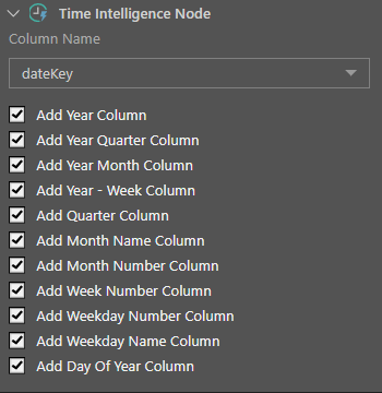
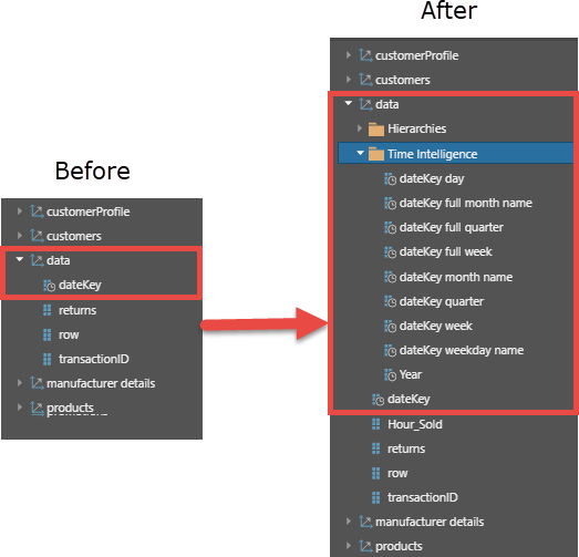
Once the node is set into a data flow, new columns are generated as shown below in the “before and after” image.
Alternatively, users can manually create custom date-time groupings using the “Calculated Columns” node and the vast date-time PQL function library. Yet another option involves using R or Python scripting to build out highly sophisticated time logic. These are more advanced choices, which I won’t cover here.
The drawback of this approach is that the results need to be stored in the database—or “materialized.” This poses issues when the data source is read-only or if the data model is meant to query the database on the fly.
If this is the case, the second option comes into play.
An on-the-fly solution is ideally suited when sourcing data from a data source when it is impossible to save a newly derived column back into the database.
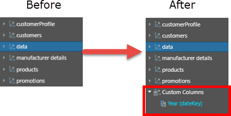
Pyramid’s Discover tool provides simple right-click functions to create and add a virtual time grouping to your data model that can be dropped and dragged into any report like its “stored” cousin.

Once the “year” option is selected, a virtual year column is created, as shown below in the “before and after” image.
While the virtual approach can offer the same outcomes as the stored approach, it comes with a few drawbacks. First, on very large datasets, its performance can be slower. Also, there are less options for creating complex time periods and setting the logic for each grouping in a different way (like “fiscal” periods).
In the end, it’s up to users to choose the method that suits them and their data, limitations notwithstanding.
The last comment in this blog covers some technical minutia. Unlike SQL-based data sources, MDX-based data models (like Microsoft OLAP or SAP BW cubes) generally should have the date-time groupings designed into the cubes natively; since it’s often impractical to add them afterwards. This does not apply to time-based calculations (like “year-to-date” or “year-on-year”)—which will be covered in my next blog.

How-To
SAP is essential enterprise software. Your organization has made significant investments in SAP. You've tailored…

How-To
Pyramid’s built-in multi-factor authentication (MFA) option adds a rock-solid layer of security to your BI…

How-To
Administrators occasionally need to check complicated settings and security structures for users. Sometimes the easiest…

How-To
Pyramid lets users customize and personalize the labels of value metrics and hierarchies for a…
How-To
Static data format masks, used to format values in analytics) is a standard feature in…

How-To
Pyramid lets users display multiple value metrics in a single report, each with its own…

How-To
Pyramid’s persistent color feature maintains the same color in all visualizations for selected data elements,…

How-To
Pyramid offers flexible, intuitive security for parent-child hierarchies, providing role-based control over how members are viewed…
How-To
Pyramid excels in its’ native support for parent-child hierarchies, automatically generating hierarchical structures and providing fluid,…